Remove outliers

The examples in this tutorial show some ways in which we can easily remove the outliers of a time series.

y = [57, 59, 60, 100, 59, 58, 57, 58, 300, 61, 62, 60, 62, 58, 57];

Indentify the outliers positions with the help of the MAD estimator (MAD = median absolute deviation = 1.4826 * median(|xi−median(x)|))

zi = (y .- median(y)) ./ mad(y)[1];

ind = abs.(zi) .> 2.5

15-element BitVector:
 0
 0
 0
 1
 0
 ...

The outliers positions are at:

outliers

2-element Vector{Int64}:
 100
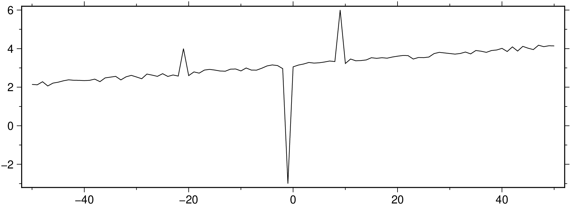
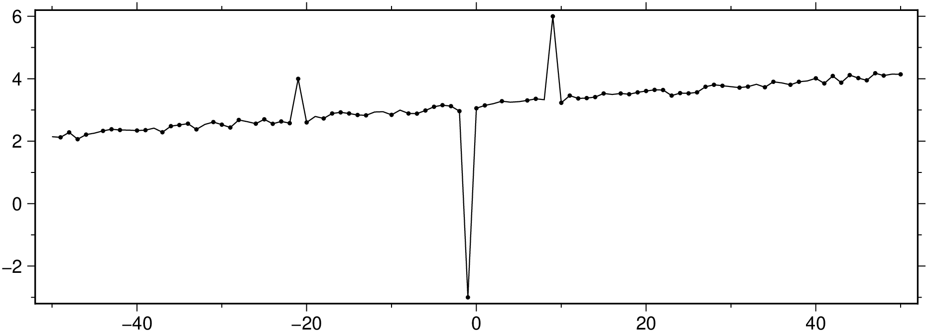
 300

x = -50.0:50;
y = x / 50 .+ 3 .+ 0.25 * rand(length(x));
# Add 3 outliers
y[[30,50,60]] = [4,-3,6];

viz(x, y, figsize=(15, 5))

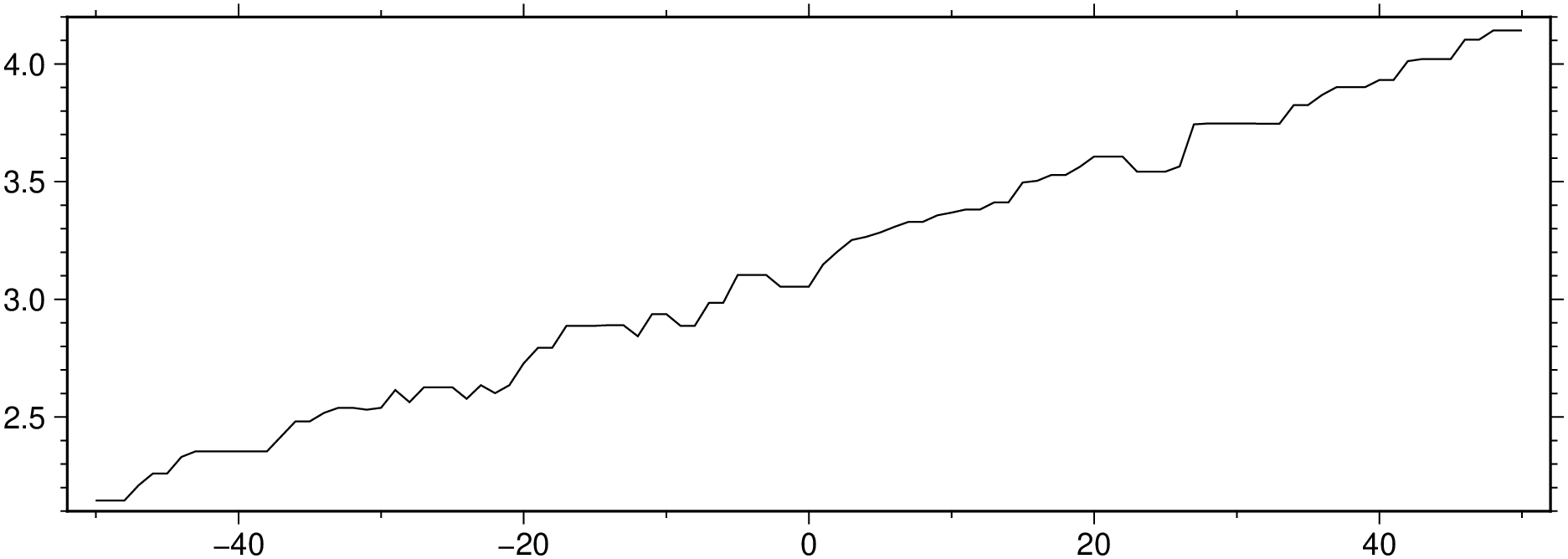
Filter out the outliers with a median filter.

D = filter1d([x y], filter=(type=:median, width=5), ends=true);
viz(D, figsize=(15, 5))

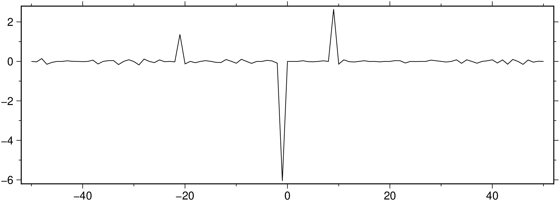
But what if we want to locale the outliers?

We can use the median filter but this time we ask filter1d do return the residues. We do that by setting the highpass option.

Dres = filter1d([x y], filter=(type=:median, width=5, highpass=true), ends=true);
viz(Dres, figsize=(15, 5))

_mad = mad(Dres[:, 2])[1] # Median Absolute Deviation

0.07313706508952521

ind = abs.(Dres[:,2]) .> 3 * _mad;
viz([x y], plot=(data=[x[ind] y[ind]], marker=:point), figsize=(15, 5))

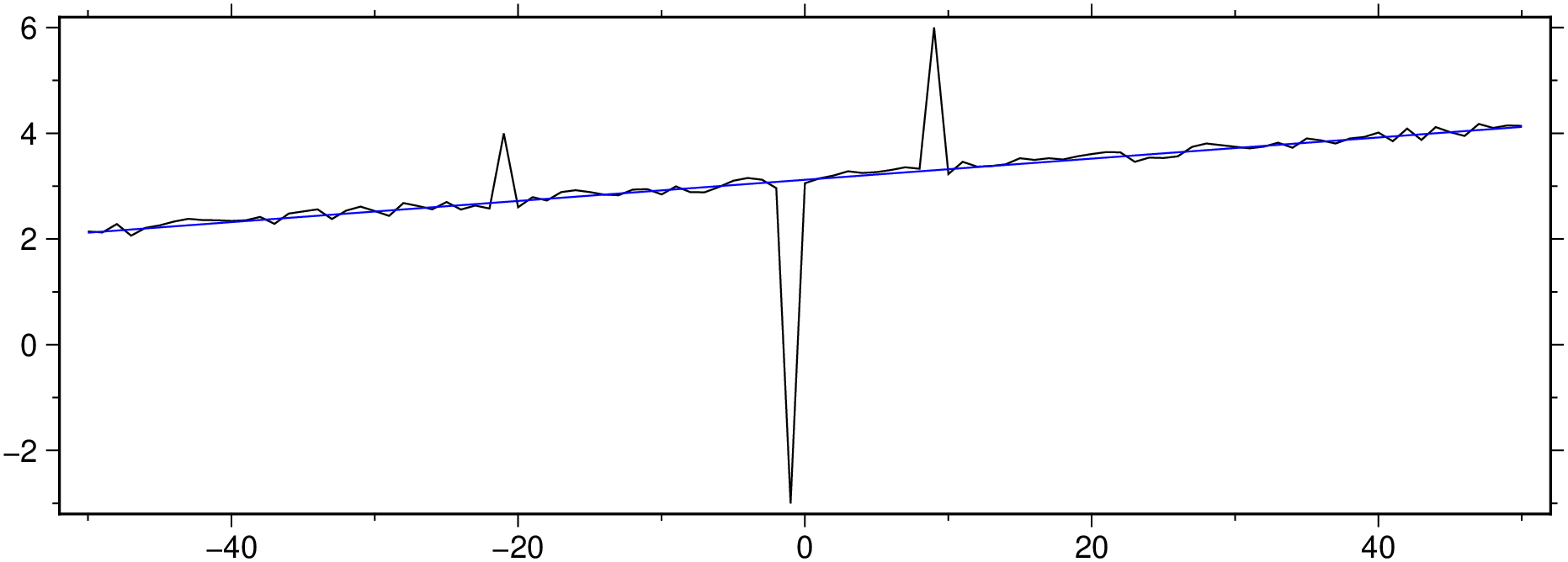
Another way

Fit a linear model and analyze the residues. The rin the out=:xmr option tells to output the residues too.

D = trend1d([x y], model=(polynome=1), out=:xmr)

BoundingBox: [-50.0, 50.0, 2.1219925238508743, 4.121792763622711, -6.101894641339074, 2.698125334683742]

101×3 GMTdataset{Float64, 2}
 Row │     x    model      residues
─────┼──────────────────────────────
   1 │ -50.0  2.12199   0.022973
   2 │ -49.0  2.14199  -0.019167
   3 │ -48.0  2.16199   0.121045
   4 │ -47.0  2.18199  -0.118259
   5 │ -46.0  2.20198   0.00810421
   6 │ -45.0  2.22198   0.0379079
   7 │ -44.0  2.24198   0.0879249
   8 │ -43.0  2.26198   0.119807
  ⋮  │   ⋮       ⋮          ⋮

D = trend1d([x y], model=(polynome=1), out=:xmr);

plot([x y], figsize=(15, 5))
plot!(D, lc=:blue, show=true)

Show the residues

viz(D[:, [1,3]], figsize=(15, 5))

mad_res, med_res = mad(D[:,3])

(0.0803265039051275, 0.0412274796762353)

zi = (D[:,3] .- med_res) ./ mad_res;
ind = abs.(zi) .> 3 * mad_res;
viz([x y], plot=(data=[x[ind] y[ind]], marker=:point), figsize=(15, 5))

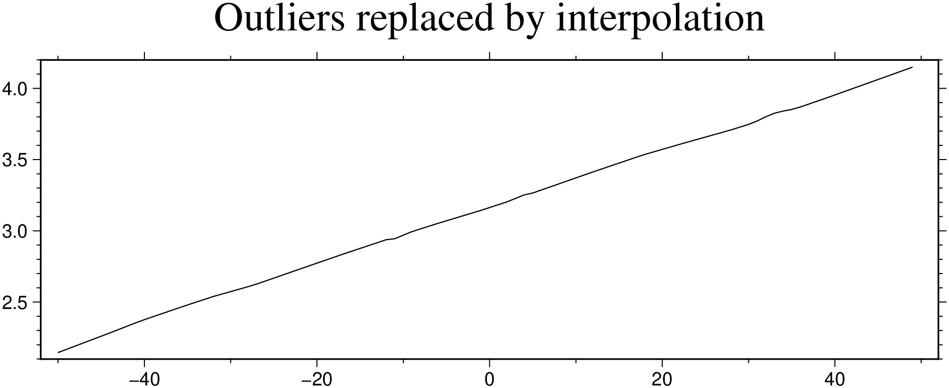
Let's replace the outliers by NaNs.

y[ind] .= NaN;

And now replace the NaNs by interpolated values.

Dfill = sample1d([x y], fill_nans=true);
viz(Dfill, figsize=(15, 5), title="Outliers replaced by interpolation")

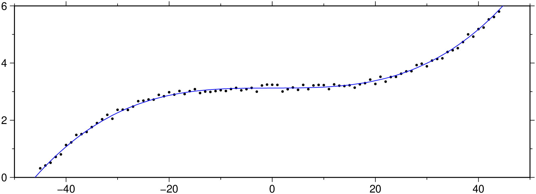
Yet another example but this time with a quadratic curve.

x = -50.0:50;
y = 4 * (x / 50) .^3 .+ 3 .+ 0.25 * rand(length(x));
D = trend1d([x y], model=((polynome=0,single=1),(polynome=3,single=true)), out=:xm);
plot(x,y, region=(-50,50,0,6), figsize=(15, 5), marker=:point)
plot!(D, lc=:blue, show=true)

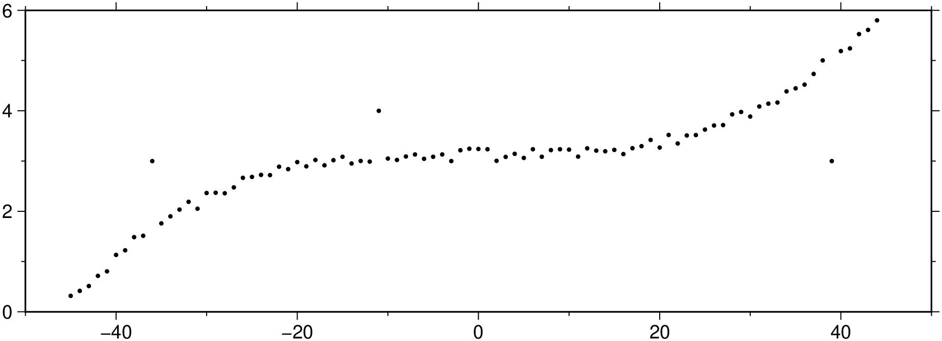
Polute it at positions [15, 40, 90].

y[[15, 40, 90]] = [3, 4, 3];
viz(x,y, region=(-50,50,0,6), figsize=(15, 5), marker=:point)

Compute and show the residues.

D2 = trend1d([x y], model=((polynome=0,single=1),(polynome=3,single=true)), out=:xr);
viz(D2, figsize=(15, 5))

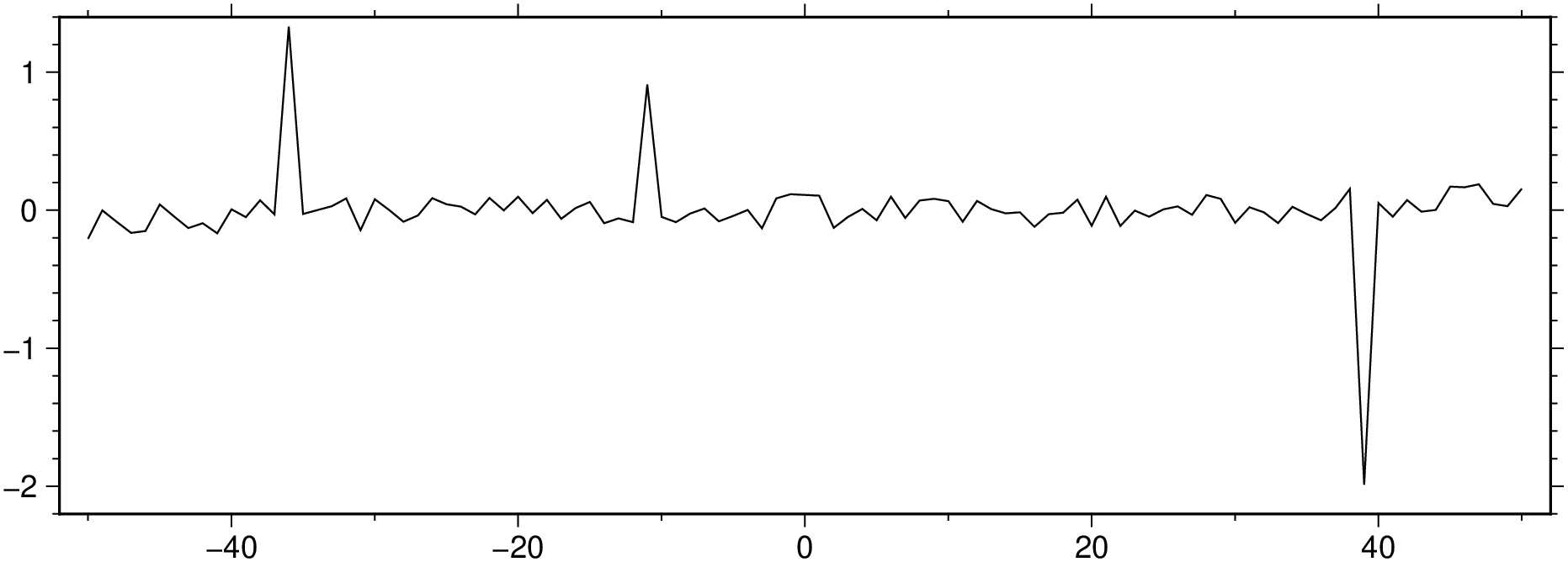
And now find the outliers positions and confirm that we obtain the locations used at the polution step.

findall(isoutlier(D2[:,2]))

3-element Vector{Int64}:
 15
 40
 90